ipywidgets demo

This example has bitrotted – see the Bokeh slider instead.

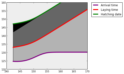
My partner Nadiah has developed an eco-evolutionary model describing the response of a migratory bird’s arrival time and prelaying period to climate change. The Octave code is here: https://github.com/nadiahpk/phenology-two-trait-migratory-bird.

The final plots look like this:

A natural question is: how does the shape of the arrival time change as the main model parameter is varied? A nice way to visualise this is using ipywidgets and nbviewer. Here is an ipython notebook with a slider for the main model parameter:

Getting this to work was surprisingly straightforward. In short:

1. Make a notebook using ipython. I used oct2py to call the Octave code from Python.

2. Install nbviewer on a publicly accessible host.

3. Run nbviewer like so:

   cd $HOME/nbviewer # this is the nbviewer repository from github
   python -m nbviewer --debug --no-cache --localfiles=$HOME/phenology-two-trait-migratory-bird
   

   This runs the server on port 5000. You could run it in a screen or tmux session, or use supervisord or angel to keep the process alive.

4. Point nginx to the nbviewer proces:

   # /etc/nginx/sites-available/amazonaws.com
   
   server {
   
           listen   80;
   
           server_name ec2-xyz.amazonaws.com;
   
           access_log  /var/log/nginx/amazonaws.com.access.log;
   
           location / {
               proxy_pass http://127.0.0.1:5000; # Reverse proxy to nbviewer
           }
   
   }
   

5. The notebook doesn’t appear on nbviewer’s front page, so just naviate to a URL of the form

   http://your.host.example.com/localfiles/foo.ipynb
   

to see the notebook foo.ipynb.