Spectral graph partitioning in Haskell

I was reading some notes from QUT about using spectral graph theory to partition a graph using eigenvalues of unnormalised Laplacian. Their Matlab code looks like this:

% Form W = Gaussian distribution based on distances
W = zeros(100, 100);
D = zeros(100, 100);

sigma = 2;
N = 100;
for i = 1:N
    for j = 1:N
        if (j ~= i)
            % Calculate the distance between two points
            dist = norm([A(i, 1) - A(j, 1); A(i, 2) - A(j, 2)]);
            expp = exp(-dist^2 / (2 * sigma^2));
            adjacency(i, j) = 1;
            % Add the weights to the matrix
            W(i, j) = expp;
            % Add up the row sum as we go
            D(i, i) = D(i, i) + expp;
        end
    end
end

L = D - W;

Find the eigenpairs of L

[vec, val] = eig(L, 'vector');
% Ensure the eigenvalues and eigenvectors are sorted in ascending order
[val,ind] = sort(val);
vec = vec(:, ind);

% Plot with clusters identified by marker
% v2
figure;
hold on;
for i = 1:N
    plot(i, vec(i, 2), ['k' plot_syms{i}]);
end

Personally, this gives me nightmares from undergrad numerical methods classes. So here’s how to do it in Haskell. Full source (including cabal config) for this post is here.

module Notes where

To create the W matrix we use buildMatrix:

buildW :: Double -> Matrix Double -> Matrix Double
buildW sigma a = buildMatrix n n $ \(i,j) -> f sigma a i j
  where
    n = rows a

    f sigma a i j = if j /= i
                        then expp sigma a i j
                        else 0.0

    dist :: Matrix Double -> Int -> Int -> Double
    dist m i j = norm2 $ fromList [ m!i!0 - m!j!0, m!i!1 - m!j!1 ]

    expp :: Double -> Matrix Double -> Int -> Int -> Double
    expp sigma m i j = exp $ (-(dist m i j)**2)/(2*sigma**2)

The D matrix is a diagonal matrix with each element being the sum of a row of W, which is nicely expressible by composing a few functions:

buildD :: Matrix Double -> Matrix Double
buildD w = diag
         . fromList
         . map (foldVector (+) 0)
         . toRows
         $ w
  where
    n = rows w

The L matrix is real and symmetric so we use eigSH which provides the eigenvalues in descending order.

lapEigs :: Double -> Matrix Double -> (Vector Double, Matrix Double)
lapEigs sigma m = eigSH l
  where
    w = buildW sigma m
    d = buildD w
    l = d - w

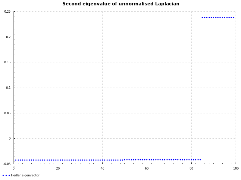
To finish up, the Fiedler eigenvector corresponds to the second smallest eigenvalue:

fiedler :: Double -> Matrix Double -> (Double, Vector Double)
fiedler sigma m = (val ! (n-2), vector $ concat $ toLists $ vec ¿ [n-2])
  where
    (val, vec) = lapEigs sigma m
    n = rows m

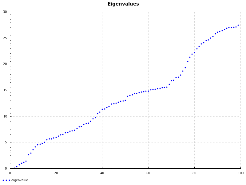
To plot the eigenvalues and eigenvector we use the Chart library which uses the cairo backend.

doPlot "eigenvalues.png" "Eigenvalues" "eigenvalue" $ zip [0..] (reverse $ toList val)

doPlot "fiedler.png"
       "Second eigenvalue of unnormalised Laplacian"
       "fiedler eigenvector"
       (zip [0..] $ toList algConnecEigVec)