Consider an option with payout on an underlying which is a cumulative sum. For example, a construction company might want to mitigate the risk of rainfall causing delays in a project. The construction company could buy a call option on the cumulative sum of rainfall not exceeding 180mm on any 3-day period. Further, we restrict this so that one day can only be used in one payoff. If the cumulative rainfall \( r \) in a 3-day period exceeded 180mm, the entity selling the call option would have the obligation to pay the construction company based on the difference \(r - 180\).
As the entity selling one of these options, we need to work out the expected loss and worst possible scenario for payouts.
Let \( r_0, r_1, \ldots \) be the sequence of daily rainfall. Form the 3-sums:
\[ s_0 = r_0+r_1+r_2, s_1 = r_1+r_2+r_3, s_2 = r_2+r_3+r_4, \ldots \]Let \(C > 0\) be the cutoff (e.g. 180mm/day). Then form the sequence \(w_0, w_1, \ldots\) where
$$ w_i = f_C(s_i) $$where \(f_C(x)\) is \(0\) if \(x \leq C\) and \(x\) otherwise.
As the seller of the option, the worst outcome for us (i.e. largest payout) corresponds to the subsequence
$$ w_{k_1}, w_{k_2}, \ldots w_{k_n} $$that maximises the sum
$$\sum_{l=1}^n w_{k_l}$$for some \(n\), where the terms \(w_{k_l}\) are mutually disjoint (i.e. we don’t take the 3-sum of any days that overlap). We consider this sum over one year, but the same approach applies to monthly, quarterly, etc.
Formulation as a graph problem Link to heading
Label vertices with the 3-sums \(w_i\) and create an edge \((w_i, w_j)\) if the sums \(w_i\) and \(w_j\) refer to overlapping time periods. Then our problem is equivalent to finding a Maximum Weighted Independent Set in the graph. This is a classic NP-hard problem.
Formulation as a linear programming problem Link to heading
Create binary decision variables \(x_0, x_1, \ldots\) and optimise
$$ \sum{w_i x_i} $$subject to
$$ x_i + x_j \leq 1 $$when \(w_i\) and \(w_j\) refer to non-disjoint cumulative 3-sums.
Python solver Link to heading
Using PuLP we can very quickly write a solver in Python.
First set up a solver:
prob = pulp.LpProblem('maxcsums', pulp.LpMaximize)
Create binary variables corresponding to each vertex:
x_vars = [ pulp.LpVariable('x' + str(i), cat='Binary')
             for (i, _) in enumerate(weights) ]
Use reduce to form the sum \( \sum w_i x_i \):
prob += reduce(lambda a,b: a+b,
                   [ weights[i]*x_vars[i] for i in range(len(weights))])
Finally, given a list of indices (3-tuples), add the constraints to avoid solutions with adjacent vertices:
for (i, x) in enumerate(indices):
  for (j, y) in enumerate(indices):
    if x < y:
      if is_adjacent(x, y):
        prob += x_vars[i] + x_vars[j] <= 1
Changi daily rainfall Link to heading
For a concrete example, let’s use the daily rainfall data for Changi in Singapore.
Here are the 3-sums:
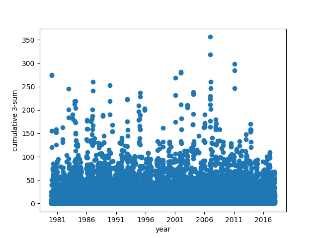
An elephant at sunset
For cutoffs from 100 to 300, here are the number of extreme events per year:
     100 120 140 160 180 200 220 240 260 280 300
1980   3   3   2   1   1   1   1   1   1   0   0
1981   1   1   1   1   0   0   0   0   0   0   0
1982   2   1   1   1   1   1   1   1   0   0   0
1983   2   2   2   2   2   1   0   0   0   0   0
1984   6   4   2   1   1   1   0   0   0   0   0
1985   1   1   0   0   0   0   0   0   0   0   0
1986   4   4   4   3   1   0   0   0   0   0   0
1987   4   3   2   2   1   1   1   1   1   0   0
1988   9   4   2   1   1   0   0   0   0   0   0
1989   3   1   1   1   1   1   1   1   0   0   0
1990   2   1   1   1   0   0   0   0   0   0   0
1991   4   3   1   0   0   0   0   0   0   0   0
1992   6   3   2   2   1   1   1   0   0   0   0
1993   1   0   0   0   0   0   0   0   0   0   0
1994   4   3   2   2   2   1   0   0   0   0   0
1995   3   3   3   2   2   2   1   0   0   0   0
1996   1   0   0   0   0   0   0   0   0   0   0
1997   0   0   0   0   0   0   0   0   0   0   0
1998   3   3   1   1   0   0   0   0   0   0   0
1999   2   0   0   0   0   0   0   0   0   0   0
2000   2   2   0   0   0   0   0   0   0   0   0
2001   5   3   2   2   2   2   2   2   2   1   0
2002   4   1   1   1   1   0   0   0   0   0   0
2003   5   1   1   1   1   1   0   0   0   0   0
2004   6   4   2   2   1   1   1   0   0   0   0
2005   2   1   1   1   0   0   0   0   0   0   0
2006   5   5   5   5   3   2   2   1   1   1   1
2007   7   5   4   3   1   1   1   1   1   0   0
2008   4   3   1   0   0   0   0   0   0   0   0
2009   1   1   0   0   0   0   0   0   0   0   0
2010   4   1   0   0   0   0   0   0   0   0   0
2011   4   2   1   1   1   1   1   1   1   1   0
2012   3   0   0   0   0   0   0   0   0   0   0
2013   5   3   3   1   0   0   0   0   0   0   0
2014   0   0   0   0   0   0   0   0   0   0   0
2015   0   0   0   0   0   0   0   0   0   0   0
2016   1   0   0   0   0   0   0   0   0   0   0
We will go with 180mm as the cutoff. Ultimately, choosing the strike is a business decision.
The burn is \(\texttt{max}(w_i - 180, 0)\), indicating the payout that the seller of the option would be liable for. Here is the daily burn for Changi daily rainfall (zero rows are not shown):
c3sum   burn
DATE
1980-01-20  275.5   95.5
1982-12-22  245.4   65.4
1983-08-22  190.6   10.6
1983-12-26  218.8   38.8
1984-02-02  219.3   39.3
1986-12-11  186.7    6.7
1987-01-11  260.5   80.5
1988-09-21  188.9    8.9
1989-12-01  252.5   72.5
1992-11-11  223.2   43.2
1994-11-11    209   29.0
1994-12-19  180.7    0.7
1995-11-02  203.4   23.4
1995-02-06  236.9   56.9
2001-01-16  268.7   88.7
2001-12-27  281.4  101.4
2002-01-25  182.1    2.1
2003-01-31  210.5   30.5
2004-01-25  237.9   57.9
2006-12-19  356.4  176.4
2006-12-26  222.7   42.7
2006-01-09  190.7   10.7
2007-01-12  260.4   80.4
2011-01-31  298.2  118.2
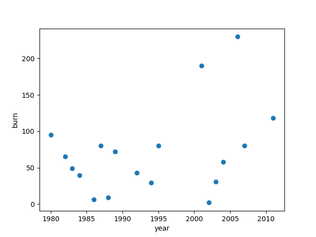
The yearly burn is \(\sum_i{\texttt{max}(w_i-180,0)}\) where the \(w_i\) are in a particular calendar year. Plotting the yearly burn:
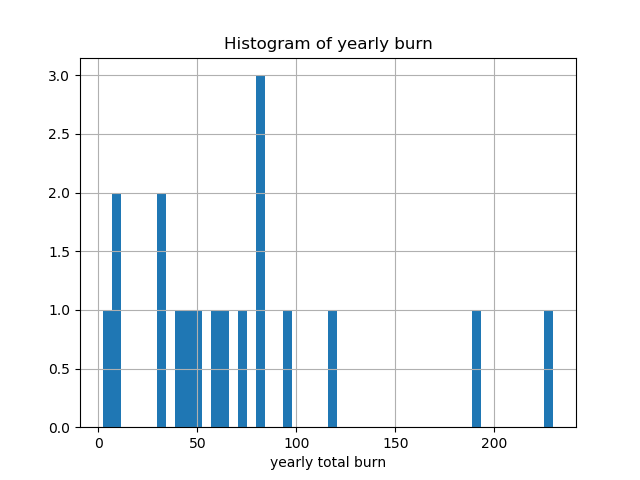
The histogram of burn values shows that a value around \(80\) is the most frequent total yearly burn:
Cumulative histogram of the yearly burn:
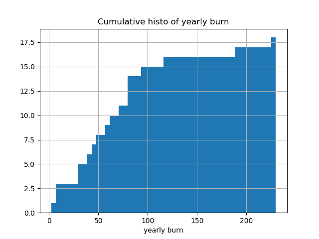
From the yearly burn we can compute the expected loss over various periods:
Expected loss (all years):     71.13
Expected loss (last 10 years): 86.22
Expected loss (last 20 years): 71.13
We see that the expected loss over the last 10, 20 years differs by about 15.0. The 99th percentile is p99 = 223.051.
Unlike pricing options on a liquid instrument such as an interest rate swap, stock, currencies, etc, the pricing of this option is set in an incomplete market. There is no way to hedge, so the Black Scholes formula cannot be used. Typically the price will be set as
$$ f(\texttt{expected loss}, \texttt{high value on the tail}) $$where the high value on the tail is p99 or p99.9 (or similar); the function \(f\) will integrate the price maker’s risk appetite, but it will be approximately
$$ \texttt{option price} \approx \texttt{expected loss} + \Delta $$Notes Link to heading
Source code is on Github: https://github.com/carlohamalainen/maxc3sum
Most of the data manipulation is done using Python Pandas which makes lots of things one-liners, e.g. to sum the daily burn to yearly burn, given an index of datetime.date, we can group by year and then sum the result:
yearly_burn = daily_burn.groupby(lambda x: x.year).sum()
To set the gap for GLPK, pass the command line option when setting up the initial GLPK object:
pulp.GLPK(options=['--mipgap', 0.1]).solve(prob)
Finding a good gap is problem-specific and requires some experimentation.